In this post, we are going to take a look at the multiple methods of evaluating flatness in GD&T and determine which is the optimal approach.
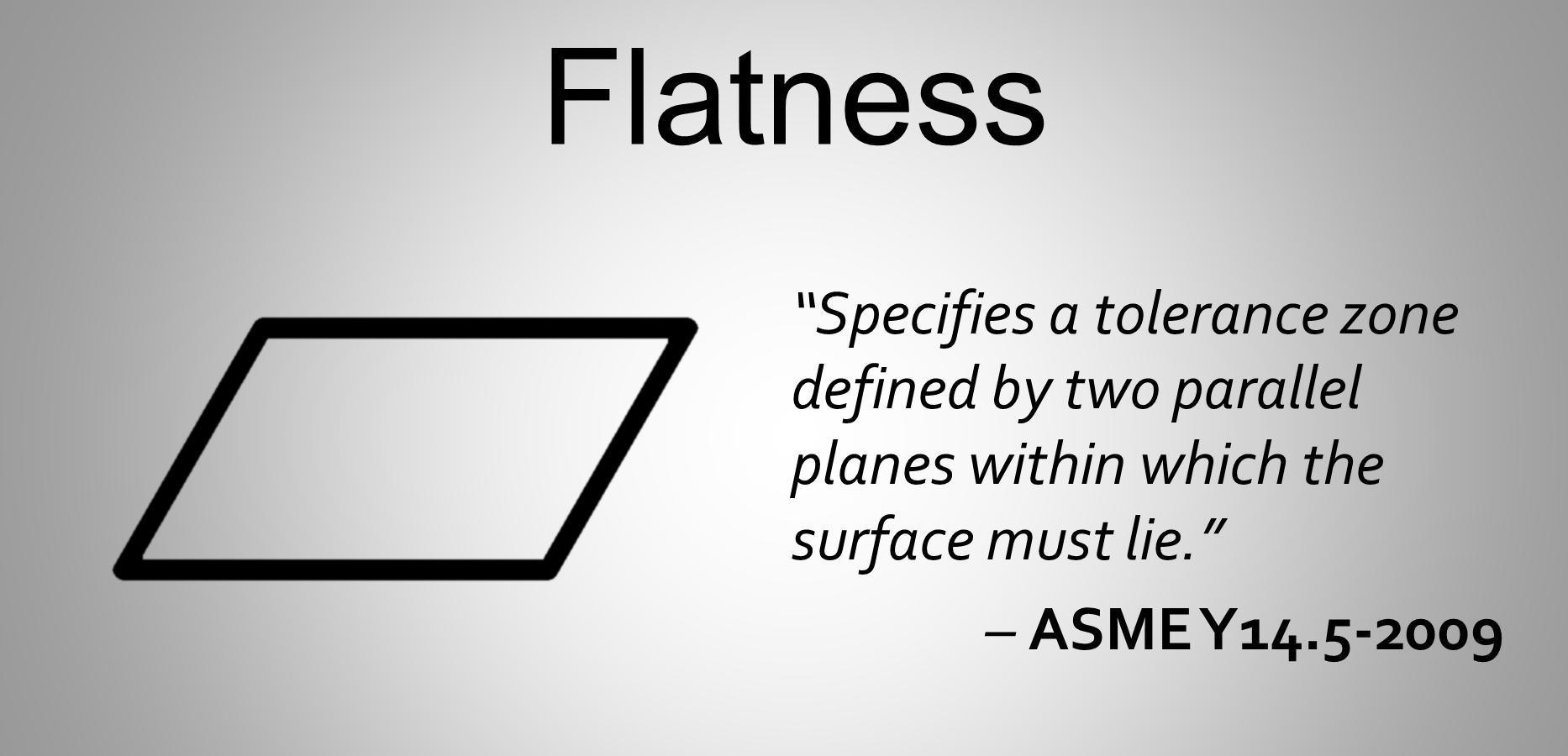
Flatness is a GD&T form tolerance that is conceptually simple. According to the ASME Y14.5 standard, it “specifies a tolerance zone defined by two parallel planes within which the surface must lie.”
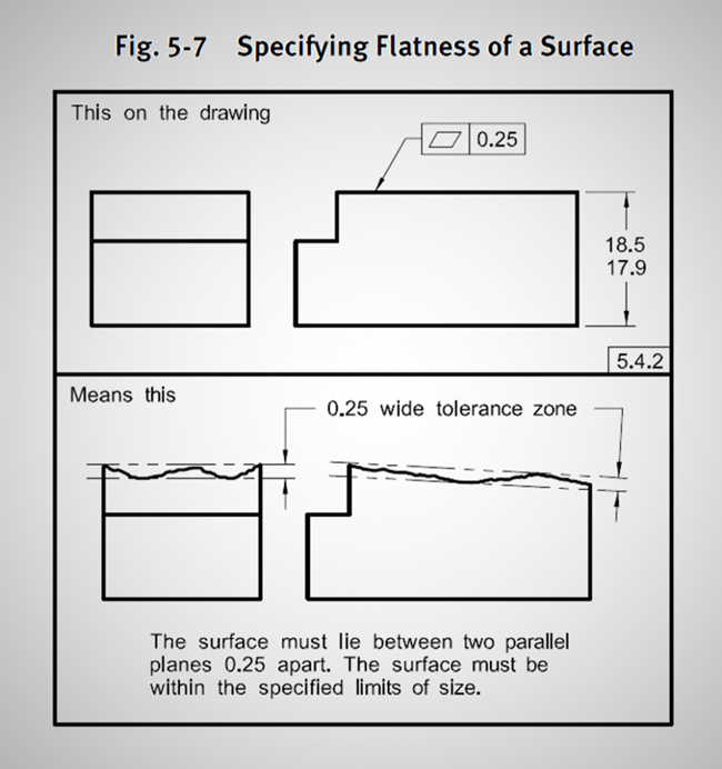
Figure 1. ASME GD&T Flatness Example
Figure 1 illustrates this concept very well. At the top, we see a drawing with a flatness tolerance of 0.25 units. According to the standard, this means that the top surface must lie entirely between two parallel planes that are at most 0.25 units apart. Picture sandwiching the surface as tightly as possible between two parallel planes; the tolerance would pass if you could get them closer together than 0.25 units. It’s important to note that the two parallel planes are not necessarily aligned with anything, as we can see in the example at the bottom of Figure 1.
Using a height gage to evaluate flatness
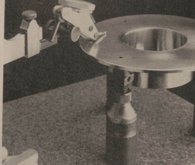
Figure 2. Height Gage on Columns set up to evaluate flatness
In application, one way to physically measure flatness is to use a height gage, as we can see in Figure 2. To use the height gage correctly, the part to be measured is first placed upon 3 columns with adjustable heights. Then, the height gage is run across the surface while looking at the amplitude of the needle. The metrologist adjusts the three columns to minimize the amplitude of the needle. They are adjusting the orientation of the plane to come up with the smallest theoretical sandwich. As you can imagine, this method requires much patience and training.
Figure 3. Using a Height Gage with the part placed directly on the surface can cause false negatives.
The more common method of using a height gage to evaluate flatness involves placing the part directly on the table (Figure 3). Without the ability to adjust the orientation of the part to minimize the amplitude of the needle, however, you are essentially evaluating parallelism based off of the table, which is sub-optimal. While it is much faster than using the 3-column method, it is important to be aware that using this method can yield false negatives; parts that pass this evaluation are always correct, but parts that fail will need to be evaluated in a different way to ensure that good parts are not sent back for expensive re-work.
Evaluating flatness using digital methods
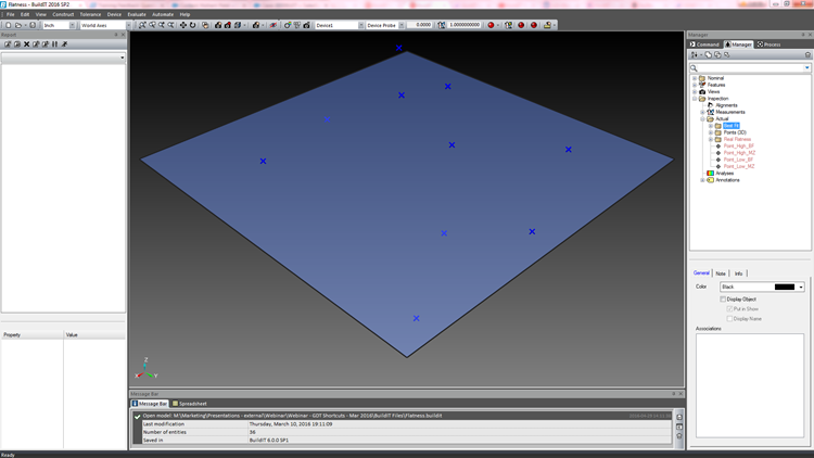
Figure 4. Surface with a GD&T flatness tolerance of 0.57 units
Let’s look at an example. We have a surface with a GD&T flatness tolerance of 0.57 units (Figure 4). In the digital realm, if you are taking measurements with a CMM (portable or otherwise), then the software has two methods of evaluating flatness: Best Fit or Minimum Zone.
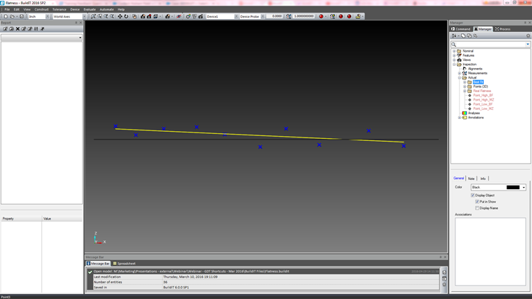
Figure 5. Best-Fit plane, as calculated through our point cloud
The Best Fit, also known as RMS plane, is an equation that will optimally fit a plane through your point cloud, finding an average while minimizing the effects of any outliers (Figure 5). The algorithm then calculates the maximum deviation above and below the fitted plane, creates two parallel theoretical planes that run through those deviations, and calculates the distance between them. This is used to evaluate the tolerance, as you can see in Figure 6.
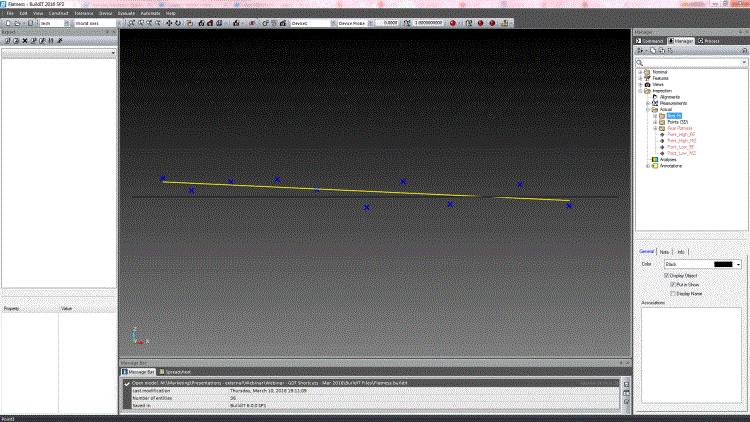
Figure 6. Best-fit plane with deviations of 0.6121 units. The algorithm calculates the maximum deviation above and below the fitted plane, marked as Point_High_BF and Point_Low_BF. It creates two parallel theoretical planes (in gray) that run through those deviations and calculates the distance between them
Similar to using a height gage without the adjustable columns, the Best Fit is a sub-optimal method of evaluating flatness in GD&T. It is also prone to false negatives. This means that it is possible to fail parts that would pass if flatness were evaluated correctly. In our example, the flatness tolerance for this plane is 0.57 units. Using the Best Fit method of evaluating flatness, the deviations come out to 0.6125 units, causing the part to fail the evaluation. This is a false negative. This is because the Best Fit plane that is created by the algorithm isn’t necessarily parallel to the two ideal planes within which the surface should lie according to the GD&T ASME standard. The orientation of the Best Fit plane is locked, removing the algorithm’s ability to adjust the sandwich to minimize the deviations. This method was used historically by metrology software because it was robust, quick and less calculation-heavy. However, with modern computing capabilities, we now have the ability to use a much better method: Minimum Zone.
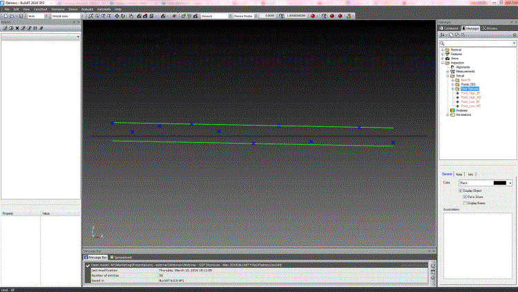
Figure 7. Minimum Zone flatness evaluation with deviations of 0.5419 units.
The Minimum Zone method of evaluating flatness in GD&T is by far the most accurate, as it is the closest to the ASME standard. Above (Figure 7), we can see that the software has created two theoretical parallel planes in green to sandwich the points as tightly as possible. Using the same example surface as above, the distance between the two planes is 0.5419 units, which would pass our tolerance of 0.57 units.
Below, Figure 8 shows the orientation differences between the sandwiches when evaluating flatness through the Best Fit and Minimum Zone methods.
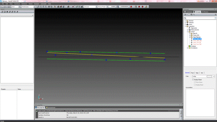
Figure 8. Comparison between the Best-Fit and Minimum Zone flatness evaluation shows the difference in orientation of the planes used to calculate the sandwich. In our example, you can also see that different high points were selected by each calculation.
Conclusion: How should you evaluate flatness in GD&T?
With the advent of digital methods of evaluating GD&T using portable CMMs and advanced 3D metrology software, there is no reason to continue to use sub-optimal or time-consuming methods. Using Best Fit to evaluate Flatness has no significant speed or resource advantages. The Minimum Zone is the optimal method as it adheres to the standard and has the added advantage of not potentially sending good parts back for expensive re-work.